Basic Shannon measures¶

The information on this page is drawn from the fantastic text book Elements of Information Theory by Cover and Thomas [CT06]. Other good choices are Information Theory, Inference and Learning Algorithms by MacKay [Mac03] and Information Theory and Network Coding by Yeung [Yeu08].

Entropy¶

The entropy measures how much information is in a random variable $X$.

\[\H{X} = -\sum_{x \in \mathcal{X}} p(x) \log_2 p(x)\]

What do we mean by “how much information”? Basically, we mean the average number of yes-no questions one would have to ask to determine an outcome from the distribution. In the simplest case, consider a sure thing:

In [1]: d = dit.Distribution(['H'], [1])

In [2]: dit.shannon.entropy(d)
Out[2]: 0.0

So since we know that the outcome from our distribution will always be H, we have to ask zero questions to figure that out. If however we have a fair coin:

In [3]: d = dit.Distribution(['H', 'T'], [1/2, 1/2])

In [4]: dit.shannon.entropy(d)
Out[4]: 1.0

The entropy tells us that we must ask one question to determine whether an H or T was the outcome of the coin flip. Now what if there are three outcomes? Let’s consider the following situation:

In [5]: d = dit.Distribution(['A', 'B', 'C'], [1/2, 1/4, 1/4])

In [6]: dit.shannon.entropy(d)
Out[6]: 1.5

Here we find that the entropy is 1.5 bits. How do we ask one and a half questions on average? Well, if our first question is “was it A?” and it is true, then we are done, and that occurs half the time. The other half of the time we need to ask a follow up question: “was it B?”. So half the time we need to ask one question, and the other half of the time we need to ask two questions. In other words, we need to ask 1.5 questions on average.

Joint Entropy¶

The entropy of multiple variables is computed in a similar manner:

\[\H{X_{0:n}} = -\sum_{x_{0:n} \in X_{0:n}} p(x_{0:n}) \log_2 p(x_{0:n})\]

Its intuition is also the same: the average number of binary questions required to identify a joint event from the distribution.

API¶

entropy(dist, rvs=None, rv_mode=None)[source]¶

Returns the entropy H[X] over the random variables in rvs.

If the distribution represents linear probabilities, then the entropy is calculated with units of ‘bits’ (base-2). Otherwise, the entropy is calculated in whatever base that matches the distribution’s pmf.

Parameters:	dist (Distribution or float) – The distribution from which the entropy is calculated. If a float, then we calculate the binary entropy. rvs (list, None) – The indexes of the random variable used to calculate the entropy. If None, then the entropy is calculated over all random variables. This should remain None for ScalarDistributions. rv_mode (str, None) – Specifies how to interpret the elements of rvs. Valid options are: {‘indices’, ‘names’}. If equal to ‘indices’, then the elements of rvs are interpreted as random variable indices. If equal to ‘names’, the the elements are interpreted as random variable names. If None, then the value of dist._rv_mode is consulted.
Returns:	H – The entropy of the distribution.
Return type:	float

Conditional Entropy¶

The conditional entropy is the amount of information in variable $X$ beyond that which is in variable $Y$:

\[\H{X | Y} = -\sum_{x \in X, y \in Y} p(x, y) \log_2 p(x|y)\]

As a simple example, consider two identical variables:

In [7]: d = dit.Distribution(['HH', 'TT'], [1/2, 1/2])

In [8]: dit.shannon.conditional_entropy(d, [0], [1])
Out[8]: 0.0

We see that knowing the second variable tells us everything about the first, leaving zero entropy. On the other end of the spectrum, two independent variables:

In [9]: d = dit.Distribution(['HH', 'HT', 'TH', 'TT'], [1/4]*4)

In [10]: dit.shannon.conditional_entropy(d, [0], [1])
Out[10]: 1.0

Here, the second variable tells us nothing about the first so we are left with the one bit of information a coin flip has.

API¶

conditional_entropy(dist, rvs_X, rvs_Y, rv_mode=None)[source]¶

Returns the conditional entropy of H[X|Y].

If the distribution represents linear probabilities, then the entropy is calculated with units of ‘bits’ (base-2).

Parameters:	dist (Distribution) – The distribution from which the conditional entropy is calculated. rvs_X (list, None) – The indexes of the random variables defining X. rvs_Y (list, None) – The indexes of the random variables defining Y. rv_mode (str, None) – Specifies how to interpret the elements of rvs_X and rvs_Y. Valid options are: {‘indices’, ‘names’}. If equal to ‘indices’, then the elements of rvs_X and rvs_Y are interpreted as random variable indices. If equal to ‘names’, the the elements are interpreted as random variable names. If None, then the value of dist._rv_mode is consulted.
Returns:	H_XgY – The conditional entropy H[X\|Y].
Return type:	float

Mutual Information¶

The mutual information is the amount of information shared by $X$ and $Y$:

\[\begin{split}\I{X : Y} &= \H{X, Y} - \H{X | Y} - \H{Y | X} \\ &= \H{X} + \H{Y} - \H{X, Y} \\ &= \sum_{x \in X, y \in Y} p(x, y) \log_2 \frac{p(x, y)}{p(x)p(y)}\end{split}\]

The mutual information is symmetric:

\[\I{X : Y} = \I{Y : X}\]

Meaning that the information that $X$ carries about $Y$ is equal to the information that $Y$ carries about $X$. The entropy of $X$ can be decomposed into the information it shares with $Y$ and the information it doesn’t:

\[\H{X} = \I{X : Y} + \H{X | Y}\]

API¶

mutual_information(dist, rvs_X, rvs_Y, rv_mode=None)[source]¶

Returns the mutual information I[X:Y].

If the distribution represents linear probabilities, then the entropy is calculated with units of ‘bits’ (base-2).

Parameters:	dist (Distribution) – The distribution from which the mutual information is calculated. rvs_X (list, None) – The indexes of the random variables defining X. rvs_Y (list, None) – The indexes of the random variables defining Y. rv_mode (str, None) – Specifies how to interpret the elements of rvs. Valid options are: {‘indices’, ‘names’}. If equal to ‘indices’, then the elements of rvs are interpreted as random variable indices. If equal to ‘names’, the the elements are interpreted as random variable names. If None, then the value of dist._rv_mode is consulted.
Returns:	I – The mutual information I[X:Y].
Return type:	float

Visualization of Information¶

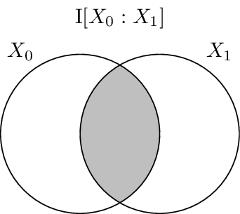
It has been shown that there is a correspondence between set-theoretic measures and information-theoretic measures. The entropy is equivalent to set cardinality, mutual information to set intersection, and conditional entropy to set difference. Because of this we can use Venn-like diagrams to represent the information in and shared between random variables. These diagrams are called information diagrams or i-diagrams for short.

This first image pictographically shades the area of the i-diagram which contains the information corresponding to $\H{X_0}$.

$The entropy :math:`\H{X_0}`$

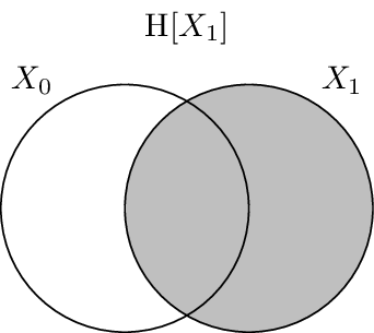
Similarly, this one shades the information corresponding to $\H{X_1}$.

$The entropy :math:`\H{X_1}`$

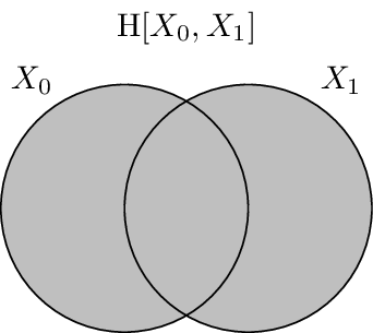
This image shades the information corresponding to $\H{X_0, X_1}$. Notice that it is the union of the prior two, and not their sum (e.g. that overlap region is not double-counted).

$The joint entropy :math:`\H{X_0, X_1}`$

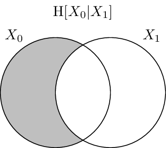
Next, the conditional entropy of $X_0$ conditioned on $X_1$, $\H{X_0 | X_1}$, is displayed. It consists of the area contained in the $X_0$ circle but not contained in $X_1$ circle.

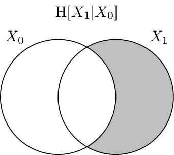
$The conditional entropy :math:`\H{X_0 | X_1}`$

In the same vein, here the conditional entropy $\H{X_1 | X_0}$ is shaded.

$The conditional entropy :math:`\H{X_1 | X_0}`$

Finally, the mutual information between $X_0$ and $X_1$, $I{X_0 : X_1}$ is drawn. It is the region where the two circles overlap.

$The mutual information :math:`\I{X_0 : X_1}`$