Information Profiles

There are several ways to decompose the information contained in a joint distribution. Here, we will demonstrate their behavior using four examples drawn from [ASBY14]:

In [1]: from dit.profiles import *

In [2]: ex1 = dit.Distribution(['000', '001', '010', '011', '100', '101', '110', '111'], [1/8]*8)

In [3]: ex2 = dit.Distribution(['000', '111'], [1/2]*2)

In [4]: ex3 = dit.Distribution(['000', '001', '110', '111'], [1/4]*4)

In [5]: ex4 = dit.Distribution(['000', '011', '101', '110'], [1/4]*4)

Shannon Partition and Extropy Partition

The I-diagrams, or ShannonPartition, for these four examples can be computed thusly:

In [6]: ShannonPartition(ex1)
Out[6]: 
+---------------------+
|  Shannon Partition  |
+-----------+---------+
|  measure  |   bits  |
+-----------+---------+
|  H[0|1,2] |   1.000 |
|  H[1|0,2] |   1.000 |
|  H[2|0,1] |   1.000 |
|  I[0:1|2] |   0.000 |
|  I[0:2|1] |   0.000 |
|  I[1:2|0] |   0.000 |
|  I[0:1:2] |   0.000 |
+-----------+---------+

In [7]: ShannonPartition(ex2)
Out[7]: 
+---------------------+
|  Shannon Partition  |
+-----------+---------+
|  measure  |   bits  |
+-----------+---------+
|  H[0|1,2] |   0.000 |
|  H[1|0,2] |   0.000 |
|  H[2|0,1] |   0.000 |
|  I[0:1|2] |   0.000 |
|  I[0:2|1] |   0.000 |
|  I[1:2|0] |   0.000 |
|  I[0:1:2] |   1.000 |
+-----------+---------+

In [8]: ShannonPartition(ex3)
Out[8]: 
+---------------------+
|  Shannon Partition  |
+-----------+---------+
|  measure  |   bits  |
+-----------+---------+
|  H[0|1,2] |   0.000 |
|  H[1|0,2] |   0.000 |
|  H[2|0,1] |   1.000 |
|  I[0:1|2] |   1.000 |
|  I[0:2|1] |   0.000 |
|  I[1:2|0] |   0.000 |
|  I[0:1:2] |   0.000 |
+-----------+---------+

In [9]: ShannonPartition(ex4)
Out[9]: 
+---------------------+
|  Shannon Partition  |
+-----------+---------+
|  measure  |   bits  |
+-----------+---------+
|  H[0|1,2] |   0.000 |
|  H[1|0,2] |   0.000 |
|  H[2|0,1] |   0.000 |
|  I[0:1|2] |   1.000 |
|  I[0:2|1] |   1.000 |
|  I[1:2|0] |   1.000 |
|  I[0:1:2] |  -1.000 |
+-----------+---------+

And their X-diagrams, or ExtropyPartition, can be computed like so:

In [10]: ExtropyPartition(ex1)
Out[10]: 
+---------------------+
|  Extropy Partition  |
+-----------+---------+
|  measure  |  exits  |
+-----------+---------+
|  X[0|1,2] |   0.103 |
|  X[1|0,2] |   0.103 |
|  X[2|0,1] |   0.103 |
|  X[0:1|2] |   0.142 |
|  X[0:2|1] |   0.142 |
|  X[1:2|0] |   0.142 |
|  X[0:1:2] |   0.613 |
+-----------+---------+

In [11]: ExtropyPartition(ex2)
Out[11]: 
+---------------------+
|  Extropy Partition  |
+-----------+---------+
|  measure  |  exits  |
+-----------+---------+
|  X[0|1,2] |   0.000 |
|  X[1|0,2] |   0.000 |
|  X[2|0,1] |   0.000 |
|  X[0:1|2] |   0.000 |
|  X[0:2|1] |   0.000 |
|  X[1:2|0] |   0.000 |
|  X[0:1:2] |   1.000 |
+-----------+---------+

In [12]: ExtropyPartition(ex3)
Out[12]: 
+---------------------+
|  Extropy Partition  |
+-----------+---------+
|  measure  |  exits  |
+-----------+---------+
|  X[0|1,2] |   0.000 |
|  X[1|0,2] |   0.000 |
|  X[2|0,1] |   0.245 |
|  X[0:1|2] |   0.245 |
|  X[0:2|1] |   0.000 |
|  X[1:2|0] |   0.000 |
|  X[0:1:2] |   0.755 |
+-----------+---------+

In [13]: ExtropyPartition(ex4)
Out[13]: 
+---------------------+
|  Extropy Partition  |
+-----------+---------+
|  measure  |  exits  |
+-----------+---------+
|  X[0|1,2] |   0.000 |
|  X[1|0,2] |   0.000 |
|  X[2|0,1] |   0.000 |
|  X[0:1|2] |   0.245 |
|  X[0:2|1] |   0.245 |
|  X[1:2|0] |   0.245 |
|  X[0:1:2] |   0.510 |
+-----------+---------+

Complexity Profile

The complexity profile, implimented by ComplexityProfile is simply the amount of information at scale \(\geq k\) of each “layer” of the I-diagram [BY04].

Consider example 1, which contains three independent bits. Each of these bits are in the outermost “layer” of the i-diagram, and so the information in the complexity profile is all at layer 1:

In [14]: ComplexityProfile(ex1).draw();

Whereas in example 2, all the information is in the center, and so each scale of the complexity profile picks up that one bit:

In [15]: ComplexityProfile(ex2).draw();

Both bits in example 3 are at a scale of at least 1, but only the shared bit persists to scale 2:

In [16]: ComplexityProfile(ex3).draw();

Finally, example 4 (where each variable is the exclusive or of the other two):

In [17]: ComplexityProfile(ex4).draw();

Marginal Utility of Information

The marginal utility of information (MUI) [ASBY14], implimented by MUIProfile takes a different approach. It asks, given an amount of information \(\I{d : \left\{X\right\}} = y\), what is the maximum amount of information one can extract using an auxilliary variable \(d\) as measured by the sum of the pairwise mutual informations, \(\sum \I{d : X_i}\). The MUI is then the rate of this maximum as a function of \(y\).

For the first example, each bit is independent and so basically must be extracted independently. Thus, as one increases \(y\) the maximum amount extracted grows equally:

In [18]: MUIProfile(ex1).draw();

In the second example, there is only one bit total to be extracted, but it is shared by each pairwise mutual information. Therefore, for each increase in \(y\) we get a threefold increase in the amount extracted:

In [19]: MUIProfile(ex2).draw();

For the third example, for the first one bit of \(y\) we can pull from the shared bit, but after that one must pull from the independent bit, so we see a step in the MUI profile:

In [20]: MUIProfile(ex3).draw();

Lastly, the xor example:

In [21]: MUIProfile(ex4).draw();

Schneidman Profile

Also known as the connected information or network informations, the Schneidman profile (SchneidmanProfile) exposes how much information is learned about the distribution when considering \(k\)-way dependencies [Ama01, SSB+03]. In all the following examples, each individual marginal is already uniformly distributed, and so the connected information at scale 1 is 0.

In the first example, all the random variables are independent already, so fixing marginals above \(k=1\) does not result in any change to the inferred distribution:

In [22]: SchneidmanProfile(ex1).draw();

In the second example, by learning the pairwise marginals, we reduce the entropy of the distribution by two bits (from three independent bits, to one giant bit):

In [23]: SchneidmanProfile(ex2).draw();

For the third example, learning pairwise marginals only reduces the entropy by one bit:

In [24]: SchneidmanProfile(ex3).draw();

And for the xor, all bits appear independent until fixing the three-way marginals at which point one bit about the distribution is learned:

In [25]: SchneidmanProfile(ex4).draw();

M-Flat Connected Informations

The Schneidman profile above walks the e-flat MaxEnt ladder (match \(k\)-way marginals, set higher-order natural parameters to zero). Amari’s dual construction walks the m-flat mixture hierarchy instead [Ama01]: distributions whose ANOVA / Hoeffding expansion of the pmf itself has no interactions above order \(k\),

\[\mathcal{M}_k = \Bigl\{ Q : Q(x) = \sum_{|S|\le k} h_S(x_S) \Bigr\}.\]

MFlatConnectedInformations (alias AmariMFlatProfile) projects \(P\) onto each \(\mathcal{M}_k\) under a chosen divergence criterion:

'jsd' (default) — Jensen–Shannon; finite on sparse supports with no smoothing
'forward_kl' — \(D(P \Vert Q)\)
'reverse_kl' — Amari’s true m-projection \(D(Q \Vert P)\) (uses symmetric \(P_\varepsilon\) / eps_schedule on sparse supports)

Profile atoms are consecutive drops in the residual to \(P\) (for reverse_kl, consecutive reverse-KL gaps between rungs, recovering the Pythagorean decomposition).

Giant Bit / Copy saturate at order 2; XOR / W need order 3.

In [26]: from dit.profiles import MFlatConnectedInformations

In [27]: from dit.algorithms import m_projection, mflat_mprojection_dists

In [28]: print(sorted(MFlatConnectedInformations(ex4, criterion='jsd').profile))
[1, 2, 3]

Helpers m_projection() / m_projection_from_subsets() and mflat_mprojection_dists() live under Optimization. The full dependency-lattice version with reverse KL is DualDependencyDecomposition.

Marginal Lift Profile

A complementary fixed-block construction: at order \(k\), form lifts of the data’s own marginals \(P_S\) (\(|S|\le k\)) plus the uniform, and fit a convex combination by least squares (MarginalLiftProfile). Coefficients show which marginals carry the approximation (Copy puts all mass on the copied pair at order 2). Unlike Amari’s free ANOVA tables, Giant Bit / XOR are not recovered from pair lifts alone — only when the full joint is an allowed block.

In [29]: from dit.profiles import MarginalLiftProfile

In [30]: copy = dit.Distribution(['000', '001', '110', '111'], [1/4]*4)

In [31]: print(round(MarginalLiftProfile(copy).residuals[2], 8))
0.0

Binding Mixture Profile

Rosas et al. [RMGJ19] distinguish collective constraints (total correlation \(T\)) from shared randomness (dual total correlation / binding entropy \(B\)). The MaxEnt Schneidman ladder decomposes the constraint face. The shared-randomness face is captured by mixtures of product distributions (latent-class / naive-Bayes models underlying Wyner common information):

\[\mathcal{F}_k = \Bigl\{ Q : Q(x) = \sum_{\alpha=1}^{k} \pi_\alpha \prod_i Q_i(x_i \mid \alpha) \Bigr\}.\]

BindingMixtureProfile fits the MLE \(Q^{(k)} = \arg\min_{Q\in\mathcal{F}_k} D(P\Vert Q)\) by EM and reports

\[\Delta B_k = B\bigl(Q^{(k)}\bigr) - B\bigl(Q^{(k-1)}\bigr)\]

(with \(B(Q^{(0)}) := 0\)). These atoms are nonnegative and sum to \(B(P)\) once the fit saturates. Giant bit concentrates at \(k=2\); XOR needs \(k=4\); copy \(X=Y \perp Z\) saturates at \(k=2\).

This is distinct from ConnectedDualInformations (still the MaxEnt ladder, only the measure is \(B\)) and from MFlatConnectedInformations (Amari additive m-flat geometry).

In [32]: from dit.profiles import BindingMixtureProfile

In [33]: from dit.algorithms import fit_mixture_of_products, mixture_of_products_dists

In [34]: gb = BindingMixtureProfile(ex2, k_max=4, n_init=8, seed=0)

In [35]: print(round(gb.profile[2], 6))
1.0

In [36]: xor_prof = BindingMixtureProfile(ex4, k_max=4, n_init=10, seed=0, early_stop=False)

In [37]: print(round(sum(xor_prof.profile.values()), 6))
2.0

Shared Randomness Decomposition

SharedRandomnessDecomposition is the dependency-lattice counterpart: at each antichain \(\pi\) the reconstruction is the product of exact block marginals (the saturated mixture-of-products model within each block, with independence across blocks), and the default atom measure is \(B\). It shares reconstructions with DependencyDecomposition but reports binding rather than entropy / total correlation.

In [38]: from dit.profiles import SharedRandomnessDecomposition

In [39]: print('B' in next(iter(SharedRandomnessDecomposition(ex2).atoms.values())))
True

Entropy Triangle and Entropy Triangle2

The entropy triangle, EntropyTriangle, [VAPelaezM16] is a method of visualizing how the information in the distribution is distributed among deviation from uniformity, independence, and dependence. The deviation from independence is measured by considering the difference in entropy between a independent variables with uniform distributions, and independent variables with the same marginal distributions as the distribution in question. Independence is measured via the Residual Entropy, and dependence is measured by the sum of the Total Correlation and Dual Total Correlation.

All four examples lay along the left axis because their distributions are uniform over the events that have non-zero probability.

In the first example, the distribution is all independence because the three variables are, in fact, independent:

In [40]: EntropyTriangle(ex1).draw();

In the second example, the distribution is all dependence, because the three variables are perfectly entwined:

In [41]: EntropyTriangle(ex2).draw();

Here, there is a mix of independence and dependence:

In [42]: EntropyTriangle(ex3).draw();

And finally, in the case of xor, the variables are completely dependent again:

In [43]: EntropyTriangle(ex4).draw();

We can also plot all four on the same entropy triangle:

In [44]: EntropyTriangle([ex1, ex2, ex3, ex4]).draw();

_images/entropy_triangle_all_examples.png

In [45]: dists = [ dit.random_distribution(3, 2, alpha=(0.5,)*8) for _ in range(250) ]

In [46]: EntropyTriangle(dists).draw();

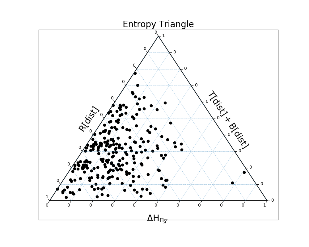
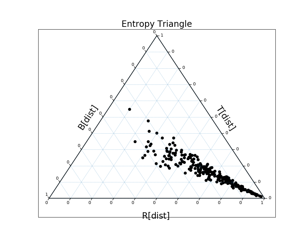
We can plot these same distributions on a slightly different entropy triangle as well, EntropyTriangle2, one comparing the Residual Entropy, Total Correlation, and Dual Total Correlation:

In [47]: EntropyTriangle2(dists).draw();

Dependency Decomposition

Using DependencyDecomposition, one can discover how an arbitrary information measure varies as marginals of the distribution are fixed. In our first example, each variable is independent of the others, and so constraining marginals makes no difference:

In [48]: DependencyDecomposition(ex1)
Out[48]: 
+--------------------------+
| Dependency Decomposition |
+---------------+----------+
|   dependency  |    H     |
+---------------+----------+
|      012      |   3.000  |
|    01:02:12   |   3.000  |
|     01:02     |   3.000  |
|     01:12     |   3.000  |
|     02:12     |   3.000  |
|      01:2     |   3.000  |
|      02:1     |   3.000  |
|      12:0     |   3.000  |
|     0:1:2     |   3.000  |
+---------------+----------+

In the second example, we see that fixing any one of the pairwise marginals reduces the entropy by one bit, and by fixing a second we reduce the entropy down to one bit:

In [49]: DependencyDecomposition(ex2)
Out[49]: 
+--------------------------+
| Dependency Decomposition |
+---------------+----------+
|   dependency  |    H     |
+---------------+----------+
|      012      |   1.000  |
|    01:02:12   |   1.000  |
|     01:02     |   1.000  |
|     01:12     |   1.000  |
|     02:12     |   1.000  |
|      01:2     |   2.000  |
|      02:1     |   2.000  |
|      12:0     |   2.000  |
|     0:1:2     |   3.000  |
+---------------+----------+

In the third example, only constraining the 01 marginal reduces the entropy, and it reduces it by one bit:

In [50]: DependencyDecomposition(ex3)
Out[50]: 
+--------------------------+
| Dependency Decomposition |
+---------------+----------+
|   dependency  |    H     |
+---------------+----------+
|      012      |   2.000  |
|    01:02:12   |   2.000  |
|     01:02     |   2.000  |
|     01:12     |   2.000  |
|     02:12     |   3.000  |
|      01:2     |   2.000  |
|      02:1     |   3.000  |
|      12:0     |   3.000  |
|     0:1:2     |   3.000  |
+---------------+----------+

And finally in the case of the exclusive or, only constraining the 012 marginal reduces the entropy.

In [51]: DependencyDecomposition(ex4)
Out[51]: 
+--------------------------+
| Dependency Decomposition |
+---------------+----------+
|   dependency  |    H     |
+---------------+----------+
|      012      |   2.000  |
|    01:02:12   |   3.000  |
|     01:02     |   3.000  |
|     01:12     |   3.000  |
|     02:12     |   3.000  |
|      01:2     |   3.000  |
|      02:1     |   3.000  |
|      12:0     |   3.000  |
|     0:1:2     |   3.000  |
+---------------+----------+

Dual Dependency Decomposition

DualDependencyDecomposition uses the same dependency lattice, but reconstructs each node by an m-flat reverse-KL m-projection rather than MaxEnt [Ama01]. At node \(\pi\) the model is

\[\mathcal{M}_\pi = \Bigl\{ Q : Q(x) = \sum_{S \subseteq T,\ T\in\pi} h_S(x_S) \Bigr\},\]

with target the symmetrically smoothed \(P_\varepsilon=(1-\varepsilon)P+\varepsilon U\) and \(\varepsilon\downarrow 0\) along eps_schedule (default (1e-4, 1e-6, 1e-8)). The default atom is \(D(Q_\pi \Vert P_\varepsilon)\) at the final eps. Symmetric smoothing preserves permutation symmetries (e.g. the W distribution), unlike random support jitter. The order-chain profile MFlatConnectedInformations is the rank-aggregated special case (all blocks of size \(\le k\)).

For the giant bit (ex2), the full pairwise cover 01:02:12 already achieves reverse KL zero. For xor (ex4), every node short of the full triple keeps a large reverse KL:

In [52]: from dit.profiles import DualDependencyDecomposition

In [53]: gb = DualDependencyDecomposition(ex2, nrestarts=4)

In [54]: pairs = frozenset([frozenset([0, 1]), frozenset([0, 2]), frozenset([1, 2])])

In [55]: print(round(gb[pairs]['rKL'], 6))
0.0

In [56]: xor = DualDependencyDecomposition(ex4, nrestarts=4)

In [57]: print(round(xor[pairs]['rKL'], 3) > 1)
True

Shapley decompositions

Ay, Polani & Virgo [APV20] assign a non-negative contribution to every non-empty subset of sources via generalized Shapley values on the input lattice.

ShapleyDependencyDecomposition decomposes \(I(\text{sources}; \text{target})\). On exclusive-or, the pair carries the whole bit and each singleton is zero:

In [58]: from dit.profiles import ShapleyDependencyDecomposition

In [59]: from dit.example_dists import Xor

In [60]: print(ShapleyDependencyDecomposition(Xor()))
+----------------------------------+
| Shapley Dependency Decomposition |
+---------------+------------------+
|   predictor   |   information    |
+---------------+------------------+
|      {0}      |      0.0000      |
|      {1}      |      0.0000      |
|     {0,1}     |      1.0000      |
+---------------+------------------+

ShapleyShannonDecomposition is an alias of the Shannon-lattice Shapley profile ShapleyDecomposition.

API

class ShapleyDependencyDecomposition(dist, sources=None, target=None, maxiter=None)[source]

Decompose I(sources; target) into non-negative Shapley-based contributions for every non-empty subset of source variables, following the method of Ay, Polani & Virgo (arXiv:1910.05979).

Each contribution I_A measures how much unique predictive information about the target is added by the subset A of source variables, averaged over all orderings consistent with the input-lattice precedence constraints.

ShapleyShannonDecomposition: alias of ShapleyDecomposition