Gács-Körner Common Information

The Gács-Körner common information [GacsKorner73] take a very direct approach to the idea of common information. It extracts a random variable that is contained within each of the random variables under consideration.

The Common Information Game

Let’s play a game. We have an n-variable joint distribution, and one player for each variable. Each player is given the probability mass function of the joint distribution then isolated from each other. Each round of the game the a joint outcome is generated from the distribution and each player is told the symbol that their particular variable took. The goal of the game is for the players to simultaneously write the same symbol on a piece of paper, and for the entropy of the players’ symbols to be maximized. They must do this using only their knowledge of the joint random variable and the particular outcome of their marginal variable. The matching symbols produced by the players are called the common random variable and the entropy of that variable is the Gács-Körner common information, \(\K{}\).

Two Variables

Consider a joint distribution over \(X_0\) and \(X_1\). Given any particular outcome from that joint, we want a function \(f(X_0)\) and a function \(g(X_1)\) such that \(\forall x_0x_1 = X_0X_1, f(x_0) = g(x_1) = v\). Of all possible pairs of functions \(f(X_0) = g(X_1) = V\), there exists a “largest” one, and it is known as the common random variable. The entropy of that common random variable is the Gács-Körner common information:

\[\begin{split}\K{X_0 : X_1} &= \max_{f(X_0) = g(X_1) = V} \H{V} \\ &= \H{X_0 \meet X_1}\end{split}\]

As a canonical example, consider the following:

In [1]: from dit import Distribution as D

In [2]: from dit.multivariate import gk_common_information as K

In [3]: outcomes = ['00', '01', '10', '11', '22', '33']

In [4]: pmf = [1/8, 1/8, 1/8, 1/8, 1/4, 1/4]

In [5]: d = D(outcomes, pmf, sample_space=outcomes)

In [6]: K(d)
Out[6]: 1.5

Note

It is important that we set the sample_space argument. If it is None then the Cartesian product of each alphabet, and in such a case the meet will trivially be degenerate.

So, the Gács-Körner common information is 1.5 bits. But what is the common random variable?

In [7]: from dit.algorithms import insert_meet

In [8]: crv = insert_meet(d, -1, [[0],[1]])

In [9]: print(crv)
Class:          Distribution
Alphabet:       (('0', '1', '2', '3'), ('0', '1', '2', '3'), ('0', '1', '2'))
Base:           linear
Outcome Class:  str
Outcome Length: 3
RV Names:       None

x     p(x)
002   1/8
012   1/8
102   1/8
112   1/8
220   1/4
331   1/4

Looking at the third index of the outcomes, we see that the common random variable maps 2 to 0 and 3 to 1, maintaining the information from those values. When \(X_0\) or \(X_1\) are either 0 or 1, however, it maps them to 2. This is because \(f\) and \(g\) must act independently: if \(x_0\) is a 0 or a 1, there is no way to know if \(x_1\) is a 0 or a 1 and vice versa. Therefore we aggregate 0s and 1s into 2.

Visualization

The Gács-Körner common information is the largest “circle” that entirely fits within the mutual information’s “football”:

Properties & Uses

The Gács-Körner common information satisfies an important inequality:

\[0 \leq \K{X_0 : X_1} \leq \I{X_0 : X_1}\]

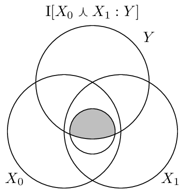
One usage of the common information is as a measure of redundancy [GCJ+14]. Consider a function that takes two inputs, \(X_0\) and \(X_1\), and produces a single output \(Y\). The output can be influenced redundantly by both inputs, uniquely from either one, or together they can synergistically influence the output. Determining how to compute the amount of redundancy is an open problem, but one proposal is:

\[\I{X_0 \meet X_1 : Y}\]

Which can be visualized as this:

This quantity can be computed easily using dit:

In [10]: from dit.example_dists import RdnXor

In [11]: from dit.shannon import mutual_information as I

In [12]: d = RdnXor()

In [13]: d = dit.pruned_samplespace(d)

In [14]: d = insert_meet(d, -1, [[0],[1]])

In [15]: I(d, [3], [2])
Out[15]: 1.0

\(n\)-Variables

With an arbitrary number of variables, the Gács-Körner common information [TNG11] is defined similarly:

\[\begin{split}\K{X_0 : \ldots : X_n} &= \max_{\substack{V = f_0(X_0) \\ \vdots \\ V = f_n(X_n)}} \H{V} \\ &= \H{X_0 \meet \ldots \meet X_n}\end{split}\]

The common information is a monotonically decreasing function in the number of variables:

\[\K{X_0 : \ldots : X_{n-1}} \ge \K{X_0 : \ldots : X_n}\]

The multivariate common information follows a similar inequality as the two variable version:

\[0 \leq \K{X_0 : \dots : X_n} \leq \min_{i, j \in \left\{0..n\right\}} \I{X_i : X_j}\]

It is interesting to note that the Gács-Körner common information can be non-zero even when the coinformation is negative:

In [16]: from dit.example_dists.miscellaneous import gk_pos_i_neg

In [17]: from dit.multivariate import coinformation as I

In [18]: K(gk_pos_i_neg)
Out[18]: 0.5435644431995964

In [19]: I(gk_pos_i_neg)
Out[19]: -0.33143555680040304

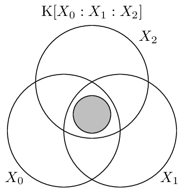
Visualization

Here, as above, the Gács-Körner common information among three variables is the largest “circle” this time fiting in the vaguely triangular Co-Information region.

API

gk_common_information(*args, **kwargs)

Calculates the Gacs-Korner common information K[X1:X2…] over the random variables in rvs.

Parameters:

• dist (Distribution) – The distribution from which the common information is calculated.
• rvs (list, None) – The indexes of the random variables for which the Gacs-Korner common information is to be computed. If None, then the common information is calculated over all random variables.
• crvs (list, None) – The indexes of the random variables to condition the common information by. If none, than there is no conditioning.
• rv_mode (str, None) – Specifies how to interpret rvs and crvs. Valid options are: {‘indices’, ‘names’}. If equal to ‘indices’, then the elements of crvs and rvs are interpreted as random variable indices. If equal to ‘names’, the the elements are interpreted as random variable names. If None, then the value of dist._rv_mode is consulted, which defaults to ‘indices’.

Returns:

K – The Gacs-Korner common information of the distribution.

Return type:

float

Raises:

ditException – Raised if rvs or crvs contain non-existant random variables.